Excel Article

Excel Tables (Part 1) - An Introduction

Over the next few articles we will explore the usage of Excel tables which are a powerful feature of Excel. We will look at when to use them and when not to use them, the advantages over using plain tables - simple ranges - and a few of the disadvantages of using them. We will also go through a practical example of building a spreadsheet to manage your current account, which will highlight many key points of using Excel tables.

There are usability advantages, such as easy filtering and sorting. But the biggest advantage is one you may not even notice, they are more robust than plain tables if built correctly. Despite the advice in the first article, it is all too easy to make mistakes with formulas and end up not applying them to all the data in the table but a subset – usually missing a few rows at the top or bottom.

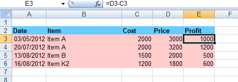
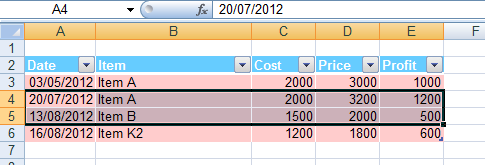
Imagine we are a retailer selling large items and recording them on a spreadsheet. We know the cost and the price after haggling but we want to know the profit.

We have created a very simple plain table and you can see how the profit is calculated, simply price minus cost.

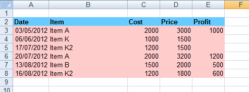
Now we add two items that we forgot into the middle of the spreadsheet, however we forget to add the formula for profit in cells E4 and E5.

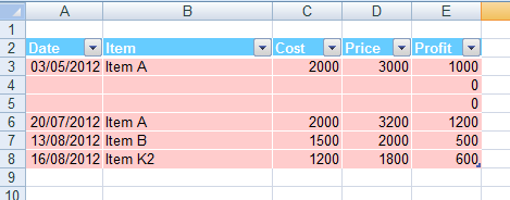
We then use the AutoSum button to generate some totals

Starting with the cost column

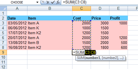
For the cost and the price gives the right result. But when we AutoSum the profit column...

...notice that the AutoSum does not pull in the whole range, only up to the blank cells. It may seem obvious in this case, but imagine you were doing this on a larger table where you cannot see the whole table, it's easy to miss.

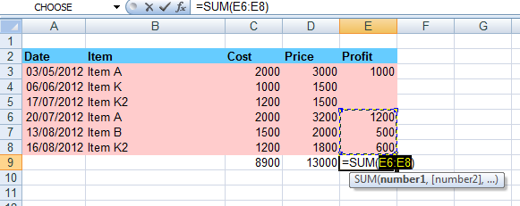
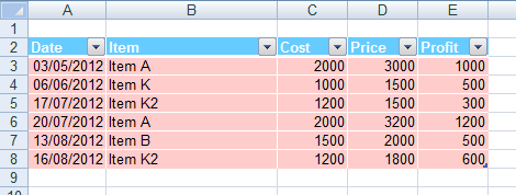
If we now enter the missing formula in cells E4 and E5

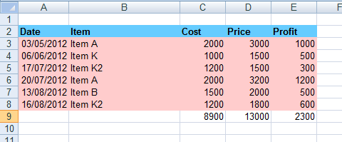
It now looks like the profit is only 2300 when it should in fact be 4100.

One solution is to avoid using the AutoSum button,or at least checking very carefully that the Sum range is correct.

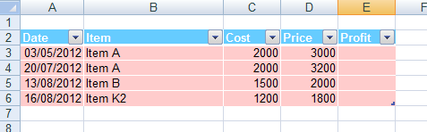
Alternatively we could use an Excel Table. Let’s rewind back to the point just before entering the profit formula, but this time using an Excel table instead.

To enter the formula, in cell E3 we type in “=”, then click on cell D3, then type in “–“ and then click on cell C3 This is the result

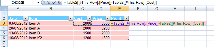
Don’t worry about the formula just yet; we will come back to that. Hit the enter key or click on the tick in the formula bar, and this is the result

Notice that column E has been filled in, with the same formula as in E2. This assumes we have “automatically create calculated columns” set to on, which is an Excel option (see below on how to check).

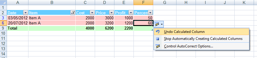
Now again we are going to insert the two missing items. We select two rows in the table.

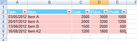
Then right click and choose insert cells above. This is the result with the profit formula already in place.

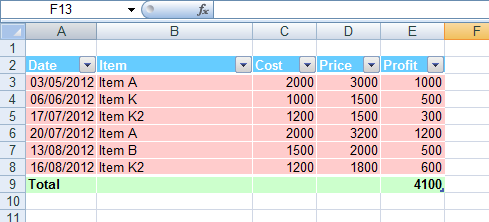
Then add the missing data. This is the result

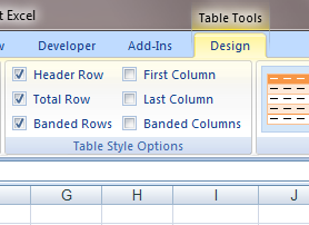
At this point we could add the totals in the usual way, using the Sum formula, but with Excel tables there is a different method we can use. With the table selected, go to table tools menu – design and tick the Total Row in the Table Style Options tab

After a spot of formatting this is the result

If you click on one of the cells in the total row, you get a drop down box

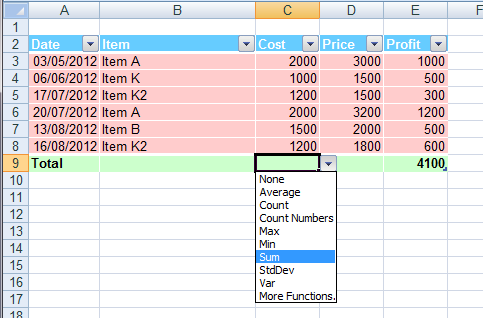
Then choose the function, you require. Note if you pick Sum from the drop down list, Excel will insert the "SubTotal" formula in. To get "Sum" you must go to "More Functions" and pick "Sum" or enter it manually.

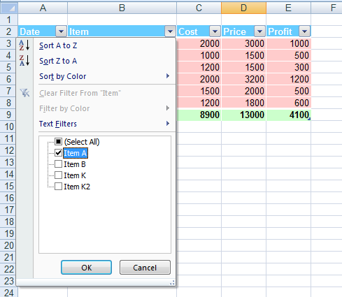
The nice thing about using the SubTotal is when you filter the table, the SubTotal will recalculate to show the total for the unfiltered figures only. For example to filter for “Item A” click on the arrow in the header row.

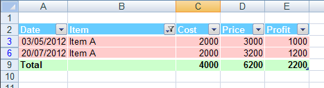
This is the result

In the next article we will look at how to create an Excel table, the components of the Excel Table and how addressing works.

Automatically create calculated columns

This feature can be turned on by going to Excel Options > Proofing > AutoCorrect options, click on the AutoCorrect Options button. In the AutoFormat as your type dialog, ensure that “Fill formulas in tables to create calculated columns” is ticked.

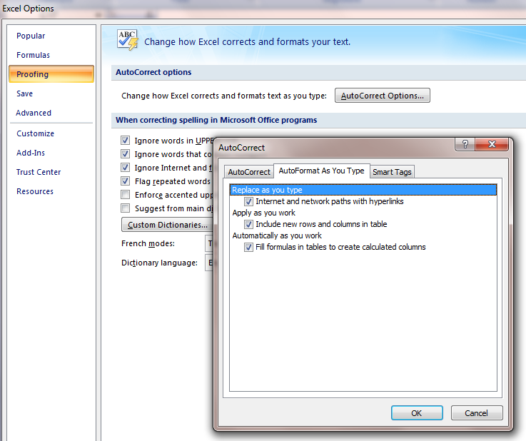
It is best to leave the option set as you can always undo a Calculated Column by clicking on the AutoCorrect options symbol (looks like a bolt of lightning).

Screen shots created in Excel 2007 on Windows 7